PDQ with MSQ Nodes

PDQ with MSQ Nodes

This page was created on April 4, 2007

1  Beta Test Distribution

Version: 4.B
Build: 041807
Languages: C only
Compiled: gcc version 4.0.0 20041026
Maintainer: Neil Gunther
If you weren't invited to come to this page, you probably shouldn't be here. In any case, caveat lector.
If you were invited, you should install the beta PDQ library in a separate directory so that nothing in PDQ 4.2 gets clobbered. Visit this page early and often and do a browser Refresh to see changes (Section 2) based on the results of other beta testers 1.

Contents

1  Beta Test Distribution
2  News
    2.1  Dateline: 10:03:59 AM Mon, Apr 16, 2007
    2.2  Dateline: 4:13:24 PM Fri, Apr 13, 2007
    2.3  Dateline: 11:56:24 AM Fri, Apr 6, 2007
    2.4  Dateline: 8:47:51 AM Fri, Apr 6, 2007
    2.5  Dateline: 1:46:41 PM Thu, Apr 5, 2007
    2.6  Dateline: 6:18:16 PM Thu, Apr 4, 2007
3  What is MSQ?
    3.1  Internet Capacity in 1917
    3.2  Morphing Approximation
    3.3  Jackson Networks
    3.4  Routed Flows in PDQ
4  Beta Testing
    4.1  Download It
    4.2  Creating an MSQ Node
5  Example
    5.1  Capacity Questions
    5.2  PDQ Code
    5.3  PDQ Report
6  Changes
    6.1  PDQ_CreateClosed()
    6.2  PDQ_CreateOpen()
    6.3  PDQ_Report()
    6.4  PDQ_Init()
7  Validations

2  News

2.1  Dateline: 10:03:59 AM Mon, Apr 16, 2007

David Marshall has suggested an interesting twist that I hadn't thought about. His idea is to leave the current CreateNode defined as it stands now, but introduce 2 new procedures: CreateMultiNode (defined on p. 226 of the Perl::PDQ book), together with CreateSingleNode (p. 228 and something I had completely forgotten about). All 3 procedures would simply provide a more flexible semantic interface for the programmer and each could be implemented with CreateNode(..., MSQ), but keeping that procedure hidden while still avoiding modifications to the solver. Sounds good to me. Comments are welcomed.

2.2  Dateline: 4:13:24 PM Fri, Apr 13, 2007

Now have MSQ running under PyDQ. You can either download the current build (see Section 4) or just do a make clean followed by a make all in the Python subdirectory.

2.3  Dateline: 11:56:24 AM Fri, Apr 6, 2007

Validated MSQ Jackson network using Example 4.2 from Gross and Harris. For more details, see model gross42.c in this distro and Section 3.4.

2.4  Dateline: 8:47:51 AM Fri, Apr 6, 2007

Updated the build and added GetVersion and passport2.c for convenience.

2.5  Dateline: 1:46:41 PM Thu, Apr 5, 2007

John Strunk has reported back that calling PDQ_Init() multiple times in the same PDQ program (Section 6.4), shows a 20× speed up in PDQ 4.B. Looks like a keeper.

2.6  Dateline: 6:18:16 PM Thu, Apr 4, 2007

Original beta build is 040407.

3  What is MSQ?

MSQ stands for Multi-Server Queue or M/M/m queue in Kendall notation. An MSQ involves a single waiting line being serviced by more than one resource. The obvious everyday example is the Post Office. A single waiting line of customers (possibly snaking out the front door because the USPS is often regarded as being notoriously slow) with the customer at the head of the line going to the next available postal clerk (as opposed to the clerk going postal on the customer 2).
The key point is that multiple servers are a natural way to model the performance of threaded applications and services that are so ubiquitous today. Each thread process corresponds to one of the M/M/m servers. Requests that cannot be processed, because all the threads are busy, must wait in a buffer or waiting line.
Here are some other examples where multi-server queues have been used: in performance models.

3.1  Internet Capacity in 1917

Of course, there's nothing new in computer science (or performance analysis).
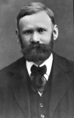
 In 1917 Agner Erlang studied "threaded servers" for the "Internet" of his day. His "Internet" was the telephone network and his "threads" were trunk lines for making calls outside Copenhagen. Trunk lines had to be reserved back then, and the telephone company wanted to know how much trunk capacity (measured today in Erlangs) they needed.
Erlang not only made the measurements, which showed the incoming teletraffic calls followed a Poisson process (i.e., Exponentially distributed interarrival periods), but he derived the very first queueing model (M/M/m, not M/M/1) in order to predict the performance (waiting time) characteristics. Not only was the first queueing model not the simplest model, but the application of probability theory must have appeared extremely novel back then (less than 100 years ago).

3.2  Morphing Approximation

Until now PDQ has only been able to solve an M/M/m node in approximation described in my Perl::PDQ book (Section 2.6.6 and Fig. 2.26). M/M/m has the morphing property that it behaves like m-parallel queues (each with mean service period S) under light traffic but, when subjected to heavy traffic, acts like an M/M/1 queue with a single server that is m-times faster than the parallel case (i.e., S/m).
What about the moderate traffic region? Well, that can be approximated quite well by R  =  [S/(1 − ρm)], the geometric residence time formula 3, where 0 < ρ < 1 is the per-server utilization (ρ = λS / m). Why the geometric approximation works at all is discussed in Section 2.6.6 my Perl::PDQ book. But this was not implemented in PDQ either. Why not? If you're going to implement M/M/m queues, you may as well solve them exactly. That's what computers are for and Erlang already published exact solutions in 1917. Moreover, an efficient iterative algorithm was developed by Jagerman in 1974, which is even more ideal for computation in PDQ.

3.3  Jackson Networks

Erlang's solution is only for a single M/M/m queue. Modern threaded applications typically involve a flow of requests between several such servers and their buffers. That's where MSQ nodes really come into their own because solving such things by hand is extremely tedious.
The most general case of an open circuit of M/M/m queueing nodes (including m = 1) is called a Jackson network. An open PDQ circuit is particularly appropriate for modeling Internet or Web applications because the total number of requests could, in principle, be unbounded. Mathematically, this is not a problem as long as the queues do not become infinite, at which point the math blows up! As a practical matter this can be a problem because real buffers have finite capacity. Buffer overflow is often associated with malicious events such as so-called "denial of service" attacks on web sites.
In other words, you might want to predict ahead of actual deployment how big a buffer needs to be. PDQ can help you there. You can examine the average wait line length (buffer size) for some peak load conditions in your PDQ model.
By definition, a Jackson network may include many M/M/m queues with various values of m, the queues may involve feedback (e.g., time-slicing which kicks the request currently being serviced off the server and back into the buffer), and it may contain multiple arrivals of work flowing in and out of the network such that the following conditions are met:
Network Traffic:
  • Requests can arrive at rates λkouter to any queueuing node k = a, b, … from outside the network
  • Requests can depart the network from any queueuing node k
  • The sum of all the arrivals (λ) into the network must equal the total departures from the network
  • The total departure rate λ is equivalent to the throughput X of the network
  • Therefore: λ = ∑k λkouter ≡ X
Node Traffic:
  • Queueuing node k can receive requests (λkouter) from outside the network
  • Queueuing node k can receive requests (λj) from any other node j = a, b, … within the network
  • The mean service time Sk is identical for all requests at node k 4
  • The fraction arriving from each node j is given by its routing probability Pjk to go from queueing node j to node k
  • By definition the routing probabilities must sum to one
  • The total departure rate from node k is the same as its local throughput Xk
  • Therefore: λk = λkouter + ∑j Pjk λj ≡ Xk
The equations above are known as the traffic equations for the network.
Jackson's theorem (J. R. Jackson 1957); notice that's 40 years after Erlang, shows that such a general network of queues can be solved as if they each queueing node was operating like an independent M/M/m queue. The PDQ model ../examples/ppa_1998/chap3/passport.c is an example of a Jackson network with m = 1 nodes that is solved using the traffic equations. This was a ground breaking result because it allowed the solution of models with multiple queues, and it is not at all obvious because the assumption of Poisson arrivals (Erlang's original assumption in Section 3.1) appears to be violated due to the possibility of feedback.
BTW: Jackson was not considering the type of data networks you're thinking about. He solved this queueing circuit 10 years before the Internet. Moreover, it had nothing to do with telephone networks or even computers. Like John D. Little, Jim Jackson was from the business managment side of the house, and he was analyzing a management scheduling problem where people are contracted for relatively short-term projects (AKA a job shop). A timeline of this and other milestones in queueing theory is presented in Appendix B of Perl::PDQ.

3.4  Routed Flows in PDQ

The discussion in Section 3.3 referred to routing probabilities (Pjk), which determine the internal flows between nodes. The question arises, how do we describe such routed flows in PDQ? The way PDQ is set up, we don't specify the local flows at each node in PDQ. All we specify is the name of the PDQ node and its associated service time. To incorporate routed flows, we use the so-called visit ratio:
Vk = λk / λ
(1)
at each PDQ node. Here's how it's done.
Consider any single-server queue labeled k in the Jackson network. In PDQ, such a node is defined by calling PDQ_CreateNode(node_k, ...), and its corresponding service time S_k is entered using the PDQ function PDQ_SetDemand(node_k, ..., S_k). For a routed flow to that node, we simply replace the service time argument by the product Vk  ×  Sk so that the call becomes PDQ_SetDemand(node_k, ..., V_k * S_k).
Using the visit ratio in this way is legitimate, as can be seen from the following proof. The mean residence time for a single-server PDQ node is given by:
Rk  =  Sk

1 − λSk
(2)
When the visit ratio in eqn.(1) is included as a factor with the service time, eqn.(2) becomes:
Rk
 = 
Vk Sk

1 − λ(Vk Sk)
 = 
λk Sk / λ

1 − λ( λk Sk /λ)
 = 
λk Sk / λ

1 − λk Sk
(3)
Subsituting Little's (microscopic) law ρk = λk Sk into eqn.(3) produces the simplification:
Rk
 = 
ρk / λ

1 − ρk
 = 
1

λ
 
ρk

1 − ρk

 = 
Qk

λ
(4)
which is equivalent to Little's (macroscopic) law Qk = λ Rk. QED.
In summary, to describe routed flows in PDQ, first calculate the visit ratio Vk for node k, using the traffic equations; numerically, this can be performed within your PDQ model. Then enter the product Vk  ×  Sk, instead of just Sk, as the service time argument viz., PDQ_SetDemand(node_k, ..., V_k * S_k) . Since the service times are the same for all requests (single class), the visit ratio simply weights the service time according to the fraction of the total flow (λ) arriving at that PDQ node.
The PDQ model passport2.c discussed on p. 95 of the Practical Performance Analyst or passport.pl on pp. 131 ff and 244 ff of Perl::PDQ, explain the visit ratio technique in more detail. The new model gross.c (included with this beta distro) demonstrates routed flows between MSQ servers.

4  Beta Testing

This section describes the new MSQ feature using an example PDQ model5.
Recognizing that the entire PDQ development effort is purely voluntary (unless anyone has some spare cash to throw at it), I don't have any particular testing schedule in mind; after all, I can't seem to keep to my own schedules when it comes to PDQ development. Hopefully, you will be sufficiently enthusiastic to try your favorite multi-server modeling ideas and report back as soon as possible.
Please be sure to report your PDQ 4.B build number against that shown in Section 1. You can run the GetVersion script to determine what it is.

4.1  Download It

Download pdq4beta.zip; the beta version of PDQ which supports MSQ. This version is an enhancement to the current 4.2 release, but it should be put into a separate directory for testing purposes.
The files are organized as: After you have unzipped the download, go into the /lib directory, select the makefile appropriate for your platform, copy it to Makefile (or copy over the one you are using in your current PDQ lib) and do a make.

4.2  Creating an MSQ Node

Currently, a queueing node is created in PDQ by calling the single-server function CreateNode(name, devtype, sched) where: are integer constants defined in PDQ_Lib.h.
To create a multi-server node, the same PDQ function is called in the usual way but contains the following parameters: CreateNode(name, m, MSQ)
MSQ (already defined in PDQ_Lib.h) tells the solver that it needs to compute performance measures for an M/M/m queue, and m is a positive integer specifying the number of servers.
We set sched to MSQ rather than devtype because the calculations in MVA_Canon.c are associated with a switch statement gated on sched. Logically speaking, MSQ is really a devtype and sched could have been assigned the number of servers, but that approach would require a rewrite of the solver.
You can only use this version with an OPEN circuit PDQ model i.e., by calling PDQ_CreateOpen, and there can only be a single PDQ stream of work. This is demonstrated in the following PDQ model involving 2 MSQ nodes in tandem.

5  Example

Big book stores, like Barnes and Noble or Borders, allow customers to enter, browse and read books, have coffee, eat, listen to CDs and finally head to the checkout area. The checkout consists of a single waiting line serviced by multiple cashiers. Such a big book store can be formally modeled as M/M/∞ (browsing) and M/M/m (checkout). The corresponding queueing diagram is shown in Figure 1. The PDQ model parameters are taken from Example 4.1 (p.170) in Gross and Harris 3rd edn. (1998) which discusses a grocery store with a "lounge". (Huh?)
Figure 1: Queueing model representation of a bookstore comprising a browsing area (M/M/∞) and a checkout area with a single waiting line (M/M/m). The corresponding PDQ code in C is shown Section 5.2.

5.1  Capacity Questions

Currently, only 3 employees are paid to act as cashiers. The capacity planning questions are as follows. If the store manager pays a 4th cashier, what happens to the:
  1. waiting time at the checkout?
  2. length of the waiting line?
  3. mean number of people in the store
The only parameter that might be made more realistic for this bookstore example, is the browsing time, e.g., increase to 65 mins.

5.2  PDQ Code

The PDQ 4.B code that corresponds to Figure 1 can be viewed in:

5.3  PDQ Report

Compiling and running the PDQ code in Section 5.2 will generate the following report as output.
Notice that in the PDQ Model INPUTS section of the report, the Node column is now used to report the number of MSQ servers (m), and the Sched column now shows that the node is a multi-server queue (MSQ). It's a hack but it works!
To address the capacity planning questions, the PDQ model is simply re-run with int cashiers = 4 and the reports compared.

6  Changes

The following is a list of changes that I have made to the PDQ 4.B source code.

6.1  PDQ_CreateClosed()

Set default work units to "Users" for TERMINAL type workloads and "Jobs" for BATCH type workloads.

6.2  PDQ_CreateOpen()

Set default work units to "Trans" for TRANSACTIONAL type workloads.

6.3  PDQ_Report()

The following changes to the PDQ reporting code will be evident when reading the output.

6.4  PDQ_Init()

Removed nested loop zeroing of arrays as requested by John Strunk of CMU on Dec 6, 2006. He will test this change to see if it offers a non-negligible speedup for PDQ models that call Init multiple times e.g., from within a loop.

7  Validations


Footnotes:

1Check the last line of this page to see the revision date of this document.
2Sorry. I couldn't resist.
3Eqn. (2.63) in the Perl::PDQ book
4A Jackson network is formally a single class (single PDQ stream) network. The extension to multiclass or multiple PDQ streams corresponds to a BCMP network.
5MSQ only works with the above 4.B PDQ library. Don't bother trying it with PDQ 4.2.
6RTT = ∑k Rk + Z = R + Z


File translated from TEX by TTH, version 3.81.
On 2 Jan 2017, 20:42.