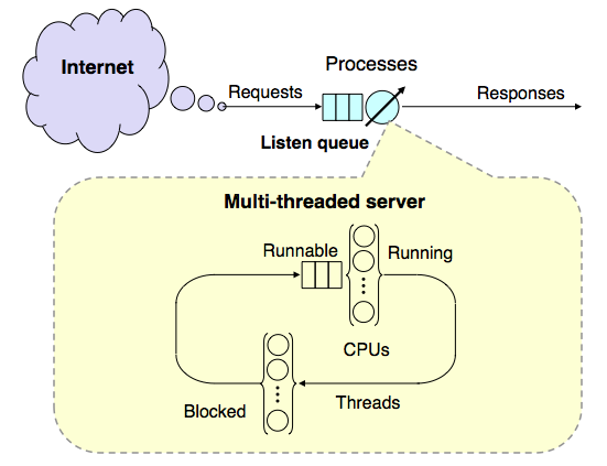
Queueing network model of a multi-threaded web service running on a multicore server
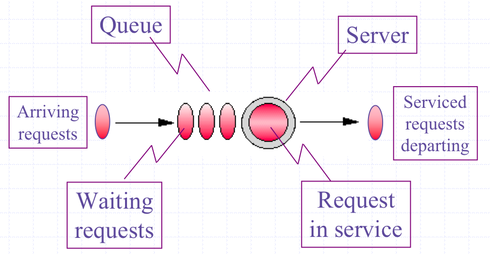
From a performance standpoint, a modern computer system can be thought of as a directed graph of individual buffers where requests may wait for service at some computational resource, e.g., a CPU processor. Since a buffer is just a queue, all computer systems can be represented as a directed graph of queues. The directed arcs represent flows between different queueing resources. PDQ computes the performance metrics of such a graph. A directed graph of queues is generally referred to as a queueing network model.
| Init() | Initializes all internal PDQ variables. Must be called prior to any other PDQ function. |
| CreateOpen() | Defines the characteristics of a workload in an open-circuit queueing model. |
| CreateClosed() | Defines the characteristics of a workload in a closed-circuit queueing model. |
| CreateNode() | Defines a single queueing-center in either a closed or open circuit queueing model. |
| SetDemand() | Defines the service demand of a specific workload at a specified node. |
| SetVisits() | Define the service demand in terms of the service time and visit count. |
| SetDebug() | enables diagnostic printout of PDQ internal variables. |
| Solve() | The solution method must be passed as an argument. |
| GetResponse() | Returns the system response time for the specified workload. |
| GetThruput() | Returns the system throughput for the specified workload. |
| GetUtilization() | Returns the utilization of the designated queueing node by the specified workload. |
| Report() | Generates a formatted report containing system, and node level performance measures. |
#!/usr/bin/perl
use pdq;
# Globals
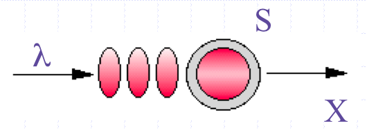
$arrivRate = 0.75;
$servTime = 1.0;
# Initialize PDQ and add a comment about the model
pdq::Init("Open Network with M/M/1");
pdq::SetComment("This is just a very simple example.");
# Define the workload and circuit type
pdq::CreateOpen("Work", $arrivRate);
# Define the queueing center
pdq::CreateNode("Server", $pdq::CEN, $pdq::FCFS);
# Define service demand due to workload on the queueing center
pdq::SetDemand("Server", "Work", $servTime);
# Change units labels to suit
pdq::SetWUnit("Cust");
pdq::SetTUnit("Secs");
# Solve the model
# Must use the Canonical method for an open network
pdq::Solve($pdq::CANON);
# Generate a generic performance report
pdq::Report();
This might look like a lot of code for such a simple model, but realize
that most of the code is for initialization and other set-up. When
amortized over more realistic computer models, that becomes a much smaller
fraction of the total code. Note also, that additional comment lines
have been included to assist you in reading this particular model.
In general, after some practice, you won't need those in every model.
                        PRETTY DAMN QUICK REPORT
               ==========================================
               ***  on   Mon Sep  7 17:19:18 2015     ***
               ***  for  Open Network with M/M/1      ***
               ***  PDQ  Version 6.2.0 Build 082015   ***
               ==========================================

COMMENT: This is just a very simple example.

               ==========================================
               ********    PDQ Model INPUTS      ********
               ==========================================

WORKLOAD Parameters:

Node Sched Resource   Workload   Class     Demand
---- ----- --------   --------   -----     ------
  1  FCFS  Server     Work       Open      1.0000

Queueing Circuit Totals
Streams:   1
Nodes:     1

Arrivals       per Secs      Demand
--------       --------     -------
Work           0.7500        1.0000


               ==========================================
               ********   PDQ Model OUTPUTS      ********
               ==========================================

Solution Method: CANON

               ********   SYSTEM Performance     ********

Metric                     Value    Unit
------                     -----    ----
Workload: "Work"
Number in system          3.0000    Cust
Mean throughput           0.7500    Cust/Secs
Response time             4.0000    Secs
Stretch factor            4.0000

Bounds Analysis:
Max throughput            1.0000    Cust/Secs
Min response              1.0000    Secs


               ********   RESOURCE Performance   ********

Metric          Resource     Work              Value   Unit
------          --------     ----              -----   ----
Capacity        Server       Work                  1   Servers
Throughput      Server       Work             0.7500   Cust/Secs
In service      Server       Work             0.7500   Cust
Utilization     Server       Work            75.0000   Percent
Queue length    Server       Work             3.0000   Cust
Waiting line    Server       Work             2.2500   Cust
Waiting time    Server       Work             3.0000   Secs
Residence time  Server       Work             4.0000   Secs
We see that the PDQ results are in complete agreement with those previously calculated by hand using the M/M/1 formulae in Section 4.1. A more detailed discussion is presented in Chapter 8 of Analyzing Computer System Performance with Perl::PDQ. Copyright © 2005—2025 Performance Dynamics Company. All Rights Reserved.