Support Materials for Dr. Gunther's CMG Presentations
Support Materials for Dr. Gunther's CMG Presentations
Contents
1 CMG 2008: Las Vegas, Nevada
1.1 A.A. Michelson Award
1.2 Sunday Workshop: How High Will It Fly?
1.3 CMG-T: Capacity Planning Boot Camp
1.4 Paper 8066: Object Measure Thyself
1.5 Paper 8143: Multidimensional Visualization of Oracle Performance Using Barry007
2 CMG 2007: San Diego
2.1 Hot Topics Session #511: Seeing It All at Once with Barry
2.2 Barycentric Coordinates Algorithm
2.3 Apdex Alliance Meeting: Triangulating the Apdex Index with Barry-3
2.4 Sunday Workshop: How to Move Beyond Monitoring, Pretty Damn Quick!
3 CMG 2006: Reno, NV
3.1 Session: Virtualization: From Hyperthreads to GRIDs
3.2 NorCal CMG Meeting in San Franscisco
4 CMG 2005: North East Regional Meetings
4.1 The Millennium Performance Problems
5 CMG 2004: Las Vegas, NV
5.1 Session #4016: Linux Load Average Revealed
6 CMG 2002: Reno, Nevada
6.1 Sunday Workshop: ASAP: Assuring Scalability for Application Performance
6.2 Session #454: Sins of Precision-Damaging Digits in Capacity Calculations
6.3 Session #681: Celebrity Boxing (and Sizing)-Alan Greenspan vs. Gene Amdahl
7 CMG 2001: Anaheim, California
7.1 Track: Website Scalability Day
1 CMG 2008: Las Vegas, Nevada
1.1 A.A. Michelson Award
If you missed my acceptance speech at the opening session on Monday evening, the slides are now available
online (PDF 3.5 MB).
In addition, TeamQuest Corporation (a major CMG sponsor)
graciously agreed to videotape my speech and this
affords a lot of opportunities to promote both CMG and TeamQuest in yet to be determined ways. Stay tuned to
my blog for updates on where the vid will appear.
Once again, I would like to publicly thank the AAM Committee, the CMG Board of Directors, and my nominators
for this honor. As I said in my speech, it really is my CMG 1993 dream come true.
1.2 Sunday Workshop: How High Will It Fly?
This workshop presented my
Universal Scalability Law (USL)
approach to quantitative scalability.
Two things I forgot to discuss:
-
Response times. Once we have calculated the USL model, we can easily compute the expected throughput
as X(p) or X(N) and from there, it is a simple matter to calculate the response times for each load level using
the formula:
This formula applies to a closed queueing-system as is valid when the load-test data is generated by a tool like LoadRunner.
-
Brooks' Law. It turns out that the USL contains
Brooks' Law as a special case.
This is not obvious because the USL expresses throughput scalability, whereas Brooks' law expresses the corresponding
latency picture.
See this blog entry
for more details.
The paper which contains the proofs of the theorems underlying the USL is available
online, but is not for the
faint of mathematical heart.
1.3 CMG-T: Capacity Planning Boot Camp
Again, I was surprised by how many people come to my CMG-T sessions. Apparently, it's a mix of both "newbies"
and "oldies" who like to hear my war stories.
Unfortunately, something got lost in the translation between my original notes and what landed on your CMG CD.
The corrected slides, including updated hyperlinks (in red), are now available as PDFs:
- Session 405: Getting Started (2.7 MB)
- Session 415: Metrics and Management (1.3 MB)
- Session 425: Going Guerrilla (1.8 MB)
If you'd like to learn more about capacity managment, come to the 2-day
Guerrilla Boot Camp class in 2009.
1.4 Paper 8066: Object Measure Thyself
This paper was presented by Michael Ducy (now at BMC Software) and Greg Opaczewski (Orbitz Worldwide)
and gave an overview of the performance monitoring architecture that has been designed and implemented at
www.orbitz.com.
It is based around their own Open Source monitoring API called ERMA
(Extremely Reusable Monitoring API), which has made their code essentially self-instrumented through the use
of frameworks, abstraction, and Aspect Oriented Programming.
Whereas we, at CMG, are usually found bemoaning the lack of application instrumentation, ERMA turns that
problem on its head and produces a veritable fire-hose of application performance data.
Then, the question becomes: What are going
to do with all that data? The authors presented one tool that they have created to address that question.
It's called
Graphite
and strikes me as MRTG/RRDtool done rigtht viz., it offers scalable images, drill down, dynamic updating, etc.
This presentation was a consequence of discussions that I had with Michael Ducy when he attended the
GBoot class earlier this year.
I then suggested that they present at CMG 2008
because they seem to have actually implemented (independently) something
that I proposed
at CMG 2002.
As became apparent after their presentation, a
lot of questions remain, so I will endeavor to establish a discussion channel for this topic which will also
enable responses from the authors.
Watch my blog for news about where this discussion
will take place.
1.5 Paper 8143: Multidimensional Visualization of Oracle Performance Using Barry007
This paper was presented jointly by Tanel Põder (an Oracle database performance expert) and myself.
It discussed the application of Barry-centric visualization (see Section 2.1) to
Oracle Wait Interface
data.
As became apparent after this presentation, a
lot of questions remain, so I will endeavor to establish a discussion channel for this topic which will also
enable responses from the author.
Watch my blog for news about where this discussion
will take place.
2 CMG 2007: San Diego
2.1 Hot Topics Session #511: Seeing It All at Once with Barry
Session 511 Monday, Dec 3, 4 pm - 5 pm
Improving data visualization paradigms for performance management is an orphaned
area of tool development. Performance tool vendors avoid investing in development
if they do not see a demand, while capacity planners and performance analysts cannot
demand what they have not conceived. We attempt to cut this Gordian knot with
Barry: a 3D performance visualization suite based on barycentric coordinates.
Potentially thousands of active processors, servers, network segments or applications
can be viewed as a moving cloud of points that produces easily comprehended
visual patterns due to correlations in the workload dynamics. Barry provides an optimal
impedance match between the measured computer system and the cognitive
computer system (i.e., your brain).
Certainly we do not understand all the neural circuitry of the brain (which appears to be a very novel kind of
non-Von Neumann parallel distributed-computer), but we do know quite a lot about certain pieces of the
brain's neural circuitry and in particular the visual system. The most recent research suggests that the retina
appears to form a sequence of
movie-like frames containing data akin to colorized
fourier transforms. A dominant feature of the brain in general, and the visual cortex in particular,
is that it is an excellent differential analyzer.
Paper (PDF)
Slides (PDF)
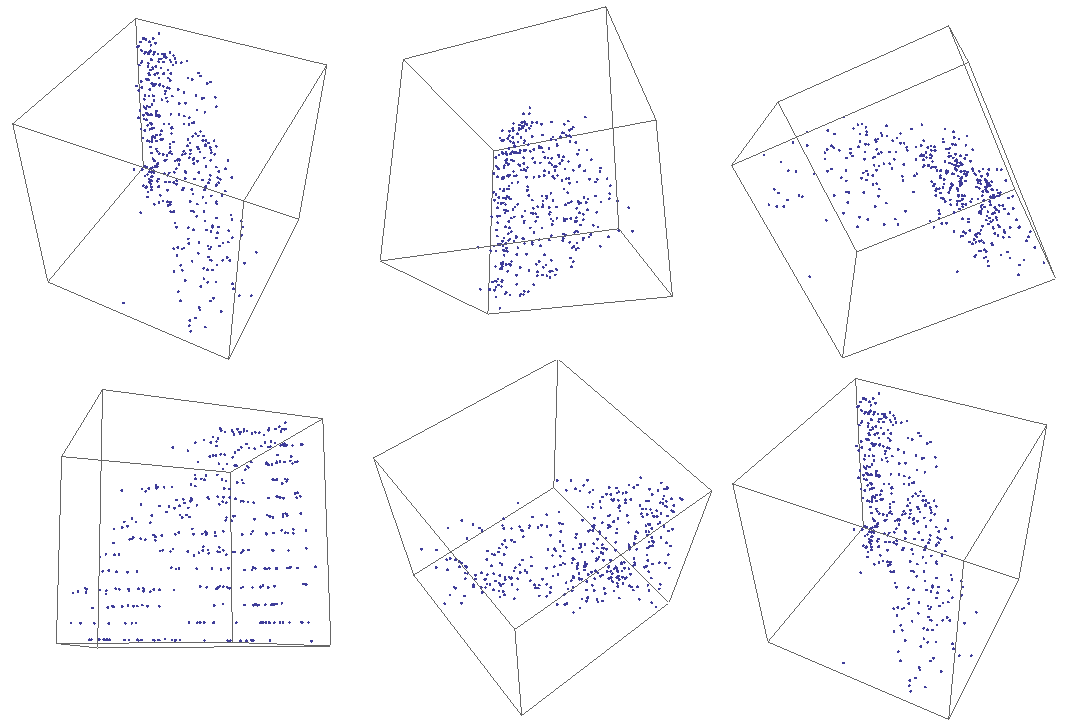
Here are some animations (created using Mathematica 6.0) of several concepts mentioned in the paper and the presentation.
| Performance Metric Eye Candy |
| MacSpin | Barry-3 | 3-Simplex | Barry4 |
 |  |  |  |
- MacSpin
- MacSpin is a facsimile of the program originally
developed for the Macintosh computer c.1988, which applied John Tukey's
concept of rotating or spinning data sets in virtual 3-space with the
mouse. The 3 attributes shown here are taken from the original CRCars
automobile data viz., horsepower, weight, model year. In general, the data
appear as a 3-dimensional scatterplot, but as the cube rotates you will see
that the otherwise random data exhibit bands at certain viewing angles.
This is not at all obvious without the ability to swivel the coordinate
system.
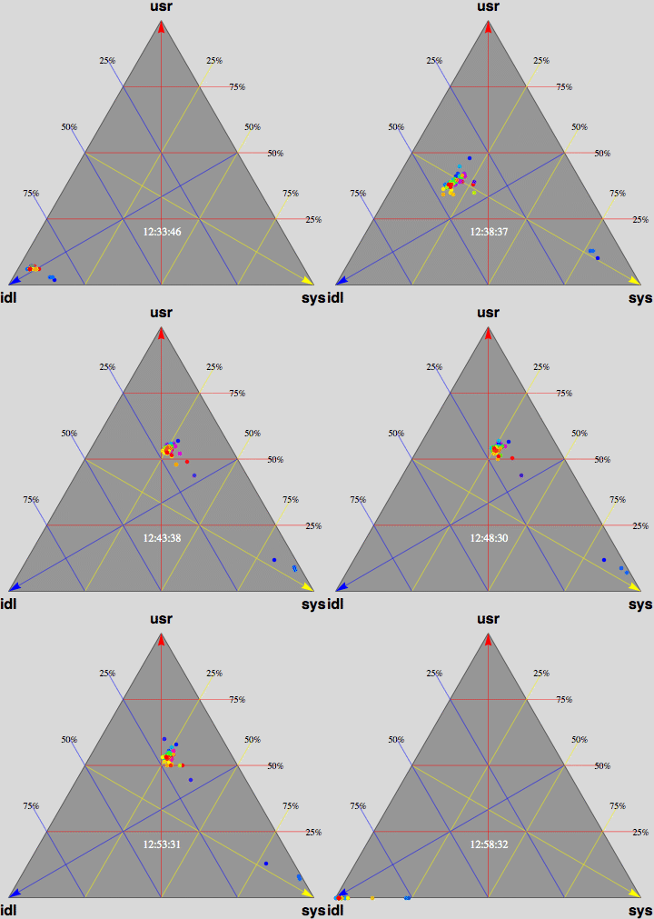
- Barry-3
- Barry-3 displays CPU utilization for a 72-way multiprocessor
running a network-based workload on ORACLE 10g. The barry-3 axes are:
- %user time (vertical upward increasing, red)
- %system time (left-right downward increasing, yellow)
- %idle (right-left downward increasing, blue)
At 12:36:46, the workload begins to ramp up starting at the lower left
corner of the triangle; maximum idleness. Most of the CPUs (shown as
colored dots) gradually make their way up the blue idle axis (decreasing
idleness) to cluster around the region bounded by the 25% idle line, the
25% sys line and the 50% usr line. However, 3 CPUs peel off at around
10% usr time and rapidly migrate (rightward) to the 80-90% sys location;
near the tip of the yellow arrow. These CPUs are dedicated to handling
network traffic and other house-keeping. At 12:53:41, the workload
completes and all the CPU dots rapidly return to the tip of the blue arrow
as they become idle again. Some clean up continues as some of the CPUs are
seen to run back and forth along the base of the Barry3 triangle (zero usr
time) between idle and system time. The frame rate of 1 second corresponds
to 10 seconds of real time, as shown in the clock display. (Data supplied
with permission by Time Cook of Sun Microsystems.)
Compare with the application of Barry-3 to the Apdex Alliance response time metrics in Section 2.3 below.
- 3-simplex
- The 3-simplex is a tetrahedron. It is formed by joining the centers of close-packed uniform spheres. Notice that all the edges between the vertices are of equal length. The 4 vertices and their opposite faces provide the basis for the barycentric coordinates. The 3-simplex enables us to display 4 degrees of freedom in 3 (virtual) dimensions; Barry4. In
our paper, we conjecture and demonstrate visually, that it is not possible to construct a Barry5 in 3-dimensions. In other words, there is no way to construct a geometric figure with all edges equal, out of close-packed uniform spheres.
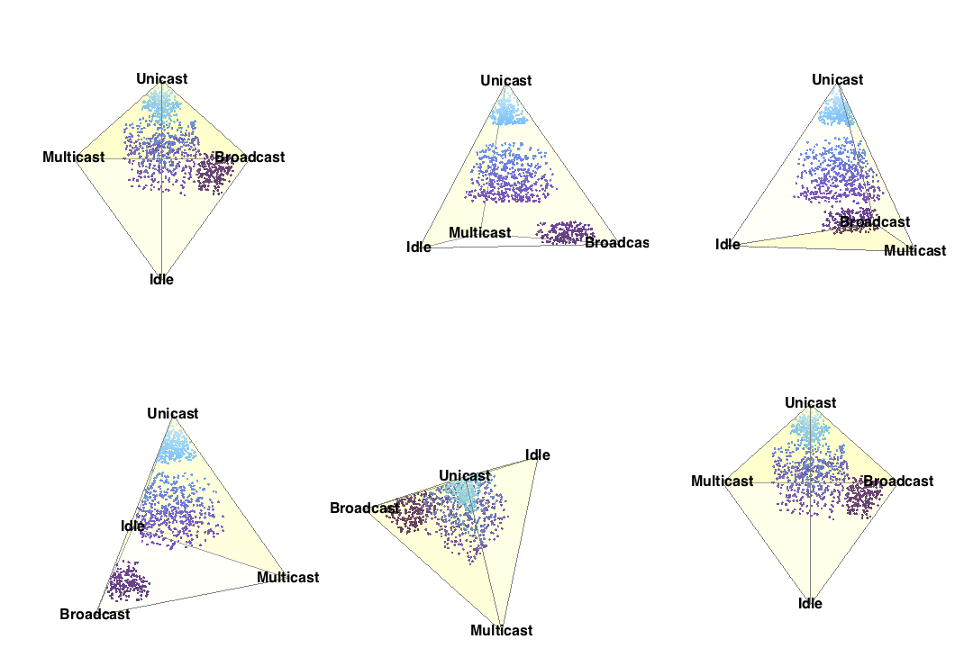
- Barry-4
- Barry-4 is an application of the 3-simplex depecting 4
network performance metrics in three dimensions for 1000 network segments
or cloud of points. It is very clear, even without looking closely at the
visual area, that the points cluster into 3 sub-clouds along certain
viewing angles. This is the barycentric analog of the MacSpin example.
2.2 Barycentric Coordinates Algorithm
Here is the algorithm for determining barycentric coordinates in
Mathematica 6.0.
Assume an equilateral triangle of unit height with its 3 vertices A, B, C organized
so that its lower left vertex is labeled 'B' at the Cartesian origin and the apex is labeled 'A'.
Then, the location of the vertices B, A, C is given by the triple:
barry3Vtx = {{0, 0}, {1/Sqrt[3], 1}, {2/Sqrt[3], 0}}
Keep in mind:
- The metrics A, B and C have to be additive in order to satisfy the sum rule requirement.
- The units of A, B and C have to be of the same type, e.g., all 'apples' or all 'oranges',
not 'apples' and 'oranges' mixed together.
Each of the barycentric axes belonging to A, B, C is normalized onto the unit interval [0, 1].
The algorithm for generating the corresponding x-y coordinates of a point within this trianglular
coordinate system is as follows.
    GetXYBarry3[Counts_List] :=
       (* Created by NJG on Thu Jun 14 14:43:19 PDT 2007 *)
       Module[
          {S, x, y, coords},
          (* Argument is a list of A, B, C Integer sample counts.
          Returns x y Real plot coordinates inside Barry triangle.*)
          If[!ListQ[Counts], Return["Error: Must be a list."]];
          If[Length[Counts] != 3, Return["Error: Must be 3 sample counts."]];
          If[!IntegerQ[Counts[[1]]] || !IntegerQ[Counts[[2]]] ||
              !IntegerQ[Counts[[3]]], Return["Error: Must be integers."]];
          A = Counts[[1]];
          B = Counts[[2]];
          C = Counts[[3]];
          S = A + B + C;
          (* A and B order swapped to position A at Barry-3 apex *)
          x = ((barry3Vtx[[1]])[[1]] * B) + ((barry3Vtx[[2]])[[1]] * A) +
              ((barry3Vtx[[3]])[[1]] * C);
          y = ((barry3Vtx[[1]])[[2]] * B) + ((barry3Vtx[[2]])[[2]] * A) +
              ((barry3Vtx[[3]])[[2]] * C);
          coords = {x/S, y/S};
          Return[N[coords]];(* Numeric rather than fractions *)
      ]
The code is fairly C-like but there are a few oddities.
- Since Mathematica is a functional programming language, even IF statements become functions.
- Curly braces {..} define a list.
- The double brackets [[..]] are the Mathematica syntax for indexing into a list.
Example:
GetXYBarry3[{132, 18, 1}] returns: {0.512351, 0.874172}
2.3 Apdex Alliance Meeting: Triangulating the Apdex Index with Barry-3
Session 45A, Wednesday, Dec 5, 4:00 PM - 5:00 PM
This is what we showed as a demonstration during our
presentation. (PDF)
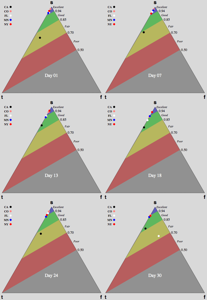
| Barry-3 Animation of Apdex Measurements |
 |
The location of each dot is determined by its percentage of satisfied
(s), tolerating (t) and frustrated (f) counts.
In this case, the unnormalized categorical data is binned according to:
- S: Samples < 4 seconds
- T: 4 seconds < Samples < 16 seconds
- F: Samples > 16 seconds
The Apdex response time measurements were collected from 5 different geographic locations (shown in the legend) over a period of 30 days.
Data supplied with permission by Peter Sevcik of the Apdex Alliance.
The gray background is superimposed to better display the colored dots.
2.4 Sunday Workshop: How to Move Beyond Monitoring, Pretty Damn Quick!
Session 191, Sunday, Dec 2, 1:00 PM - 4:30 PM
PDQ models (zip)
Included files are:
| baseline.c | Baseline for 3-tier client-server architecture |
| cpuGrowth.py | Growth model for CPU utlization and load average in PyDQ |
| ebiz_naive.c | Basic 3-tier web application model |
| ebiz_retro.c | Web application model including retrograge throughput |
| Makefile | Make file for PDQ models written in C |
| mm1_ok.py | Simple M/M/1 queueing model in python |
| mm1.pl | Simple M/M/1 queueing model in Perl |
| scaleup.c | Increase client load for 3-tier client-server architecture |
| upgrade1.c | Upgrade scenarios for 3-tier client-server architecture |
| upgrade2.c | More upgrade scenarios for 3-tier client-server architecture |
3 CMG 2006: Reno, NV
3.1 Session: Virtualization: From Hyperthreads to GRIDs
A HREF="http://www.perfdynamics.com/Papers/njgCMG06.pdf">Paper (PDF)
3.2 NorCal CMG Meeting in San Franscisco
I want to thank everyone who attended the
Northern California CMG
kick-off meeting for 2006, sponsored by SAS Institute in San
Franscisco. Cathy Nolan did a great job of organizing, as usual. I
really enjoyed giving the presentation, and I hope you enjoyed it half
as much as I did! Some of you asked such insightful questions that I
will now have to make some more edits to my Guerrilla Capacity
Planning
book.
Better now than later!
Toward the end of my presentation, a young lady in the front row asked
me about applying my Universal Scalability Law to
multi-tier architectures. I appeared to "page fault" on the
question. That's because I did! What is really weird is, that I already
have a section in my presentation where I discuss that topic but I
skipped it because we were running short on time. Since I forgot that
section was included, I ended up trying to recall another client-server
architecture that I had been working on a few months ago, and that's why
I was busy "paging in". (Well, that's my story and I'm sticking
to it! ;-)) Anyway, the answer it, Yes (see the slides).
Here are the materials you requested:
- Download my presentation
"Scalability on a Stick"
(PDF 5MB).
- The queueing theorem I discovered (that got panned by many "parallel people") can be stated thusly:
Amdahl's law for parallel speedup is equivalent to the synchronous queueing
bound on throughput in the repairman model of a multiprocessor.
It was first published on
arXiv
in 2002. It provides the justification for applying the same Universal Scalability Law
to both software and hardware systems.
The Repairman queueing model is discussed in my "Perl PDQ"
book.
My theorem has recently been demonstrated by my colleague
Prof. K. J. Christensen
to be correct using simulation and is currently being written up more formally for journal publication.
- The new Guerrilla
book
(due out summer 2006) will contain 3 chapters on the
Universal Scalability Law.
- In the meantime, check out
The Guerrilla Manual
online, and have some fun with you manager and colleagues.
- You might also get your manager to pay for a Guerrilla
training class.
- Download an EXCEL
spreadsheet
containing universal scalability models for both hardware and software.
- Feel free to
contact me
if you have any other questions or comments.
4 CMG 2005: North East Regional Meetings
At the local CMG meetings in Boston and Hartford, I gave a talk entitled
The Millennium Performance Problems, and it seems to have generated
a lot of interest. What follows is a brief discription of that talk.
4.1 The Millennium Performance Problems
This material is based on a keynote presentation I gave at the
TeamQuest
User Group meeting during CMG 2004 in Las Vegas, Nevada.
A later version was presented as a Webinar sponsored by TeamQuest.
The Millennium Performance Problems are:
- Performance Visualization:
The idea here is to find ways of representing performance data that are
a better impedance match for our cognitive computer (our brain). One
role model is the techniques used in so-called Scientific
Visualization where physicists and biologists have learned to use
things like special GUIs and animation to represent complex data in ways
that help them solve problems. Why should they have all the fun?
- Self-instrumented Applications:
Object-oriented programming has been promoted as a good thing primarily
for reasons of reusability. If people are going to re-use objects, how
about they come with their own instrumentation? This really should be
part of the object library so that a programmer need nevre be concerned
with adding such code. Then I, as the performance analyst would have the
ability to turn objects on selectively and thereby trace paths through
application code to find bottlenecks, even on production systems.
- The Von Neummann Bottleneck:
An efficient way to compute something on a machine is to do more than
one thing at once. The technical term is parallelism.
Unfortunately, despite a lot of intense effort over the last two
decades, general-purpose parallelism remains a holy grail of performance
analysis. One reason for this barrier seems to stem from the influential
success of early electronic computer designers such as Alan Turing and
John von Neumann. The fundamental paradigm of sequential programming and
operation seem to be almost impossible to break away from in the modern
digital computer. But there is an obvious role model for a non-von
computer architecture: our brain. This has led to the idea
neural networks as way of achieving a higher degree of
parallelism. Quantum computers are another.
- Performance Analysis of the Internet:
The results of analyzing Internet packet traces 15 years ago at Bellcore (now
Lucent) showed that long-term correlations can persist over several
orders of magnitude in time. Packet arrivals are not Poisson, and
service times are not constant. In other words, all the conventional
queueing theory techniques near and dear to our hearts as performance
analysts, are no longer valid at the packet level. How are we to model the
Internet? Perhaps we need to think big. The climatologists use things like
the
Earth Simulator
to address complex questions about global warming. Maybe we need an Internet Simulator of similar scale?
- Performance Analysis of Quantum Computers:
Quantum Computers are probably a long way off, but
quantum communication devices
are already here. The only reason you are not aware of them is because they are expensive and therefore
a specialty item for institutions like banks. In the next 3 to 5 years, I believe these things will
reach commodity prices and will therefore become more ubiquitous.
I am also working on these
technologies
now. The question for us is, How will they affect performance?
If you have questions or other ideas about important performance issues, please send your
comments
by email and I will consider adding them here.
5 CMG 2004: Las Vegas, NV
5.1 Session #4016: Linux Load Average Revealed
- Download the
handout (PDF)
(which wasn't available at the session)
- This topic is also covered in Chap. 4 of my new book
Analyzing Computer System Performance wih Perl::PDQ
(Springer-Verlag, 2005) which includes examples and problems as well (ISBN: 3540208658)
- Linux Load Average Reweighed Following my presentation,
someone asked me over lunch how the weight factor
exp(-5/60) arose in either the Linux code or my paper. The
explanation turns out to be almost another paper in its own right!
Soon, I will post my analysis on the Web. Watch this space for details.
6 CMG 2002: Reno, Nevada
6.1 Sunday Workshop: ASAP: Assuring Scalability for Application Performance
- Sunday
schedule
- Download
corrected tutorial slides
- Sample scalability (EXCEL)
spreadsheet
- Attendee Comments:
- Jim Holtman (Convergys): Informed me that the free software package called
"R"
can solve my
super-serial equation
directly from the (uninverted) scaling measurements.
"R" is a subset of the commercial (and expensive)
S-PLUS
programming language. Amusingly, I've had this
package installed on my laptop but never found time to learn to use it.
- NJG: I mentioned that
Mathematica
can also solve my nonlinear super-serial equation directly. Another free software package called
Octave (more like Matlab than Mathematica)
may be able to do this but I haven't tried it.
6.2 Session #454: Sins of Precision-Damaging Digits in Capacity Calculations
- Invited Speaker Session
- Tools
(in VBA, Perl, and Mathematica) accompanying this session.
- SAS Anyone?
I don't do SAS but a member of the audience kindly offered to
provide a SAS version of the SigFigs code. Please
contact
me when it becomes available. I will post it with full attribution for your work. Thank you.
- Answers to Quiz:
| Significant Figures | Rounding Problems |
| Problem | Answer | Value | Problem | Answer | Value |
| 1 | (e) | 0.00030 | 1 | (e) | 0.8 |
| 2 | (e) | five | 2 | (d) | 42.3 |
| 3 | ?1 | none | 3 | (d) | 10.3 |
- Ambiguous cases that arose during the presentation:
- How many sigfigs in 3600 seconds?
If we simply apply the rules as presented the answer would be 2 sigfigs.
On the other hand, 3600 seconds (per hour) comes from the fact that
1 minute has 60 seconds (1 sigfig) and 1 hour has 60 minutes (1 sigfig). Using the
"Golden Rule" requires that 60 * 60 = 3600 should be written as 4000 (i.e., rounded up to 1
sigfig; matching the multiplicand with the least significant digit).
It seems that numbers like 3600 seconds per hour are defined constants,
not measured values. Therefore, in any calculation, it should be written explicitly as
3600•
i.e., with the implicit decimal point made explicit. Otherwise, we might not know that
it represents a defined constant with 4 sigfigs and treat it as a measured value with only 2 sigfigs.
- How many sigfigs in 0.0 ?
Still undecided about this one. Is the second zero a leading or trailing zero?
Certainly there are occasions when one would want to indicate that the
measured value was zero to 1 decimal place (in which case it would be considered to express 1 sigfig
of accuracy).
If you have any constructive comments that might advance these issues, please
contact me
and I will add your remarks.
6.3 Session #681: Celebrity Boxing (and Sizing)-Alan Greenspan vs. Gene Amdahl
7 CMG 2001: Anaheim, California
7.1 Track: Website Scalability Day
Copyright © 2001-2008 Performance Dynamics Company. All Rights Reserved.
Footnotes:
1As pointed out by Jim Gonka, there was a line missing from this question.
File translated from
TEX
by
TTH,
version 3.38.
On 26 Jul 2011, 08:36.
